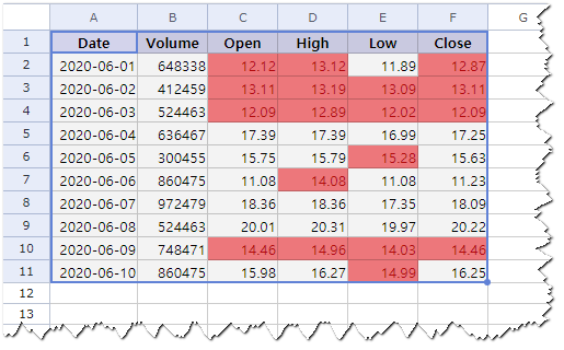
Values within the specified range are highlighted with the formatting.
Find and format cells that meet the specified condition. Conditional Formatting makes it easy to identify data by highlighting cells or ranges of cells that meet certain conditions. You can also apply a data bar or icon and use the hue function to easily analyze your data.
Perform the following to change the data display format.
Perform the following to apply the top rule.
Perform the following to clear conditional formatting applied to a cell.
Perform the following to modify conditional formatting.
The submenu of Format-Conditional Formatting are as follows:
Highlight a cell that meets the condition. Please note that the preview images listed in Color Scales do not represent the actual effect.
Use for a statistical condition in relation to other values.
Use for a value comparison using gradient-filled horizontal bars in different length.
Highlight cells with different fill colors to ranges of value data.
Use to rank the cell contents into 3 to 5 categories.
You can clear conditional formatting from cells or worksheet.
You can define and add new rules and you can delete them at any time. The rules you define can be modified or deleted as you need or want.
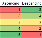
The preview images listed in Conditional Formatting-Color Scales do not represent the actual effects and are applied differently depending on the size of the cell data. For example, if you have data in ascending or descending order, applying the same color will have different results as in the example below.